IndeX-Ray™: Imaging Technology for Database Indexes

Here at Query Doctor (find us on Discord) we are big fans of visualizations and of mental models. Together these two techniques allow complicated concepts to be easily understood. Applying this to indexes specifically is one of the superpowers that makes our doctors so effective.

A data structure known as a B+ tree is what the majority of database indexes are built on today. The details of such data structures are interesting and there are many resources available online if you want to dive into them in full. As it turns out for our purposes though, there are only a few key facts about them that need to be known in order to build a robust model for using them. Those concepts are:

• The tree has a well-defined order which is declared when the index is created.
• All of the user data is available in the final layer of the index which we call the leaf nodes.
• The leaf nodes all point to their neighbors.

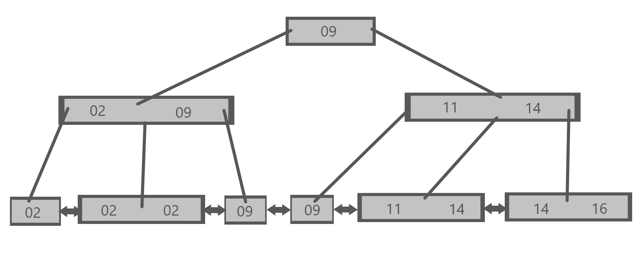
In "reality", a typical B+ tree may "look" like this:

By contrast, here is how we think about the same structure:

There are some obvious differences between these structures which we will explore momentarily. Despite those differences, notice that our model preserves the three critical components of B+ trees mentioned above. We can see, for example, that the values in the leaf nodes are ordered in the same way.

So if these two representations are the same in those important ways, what is the point of offering an alternative at all? An example should help.

Example: Finding High Scores

Consider the following query:

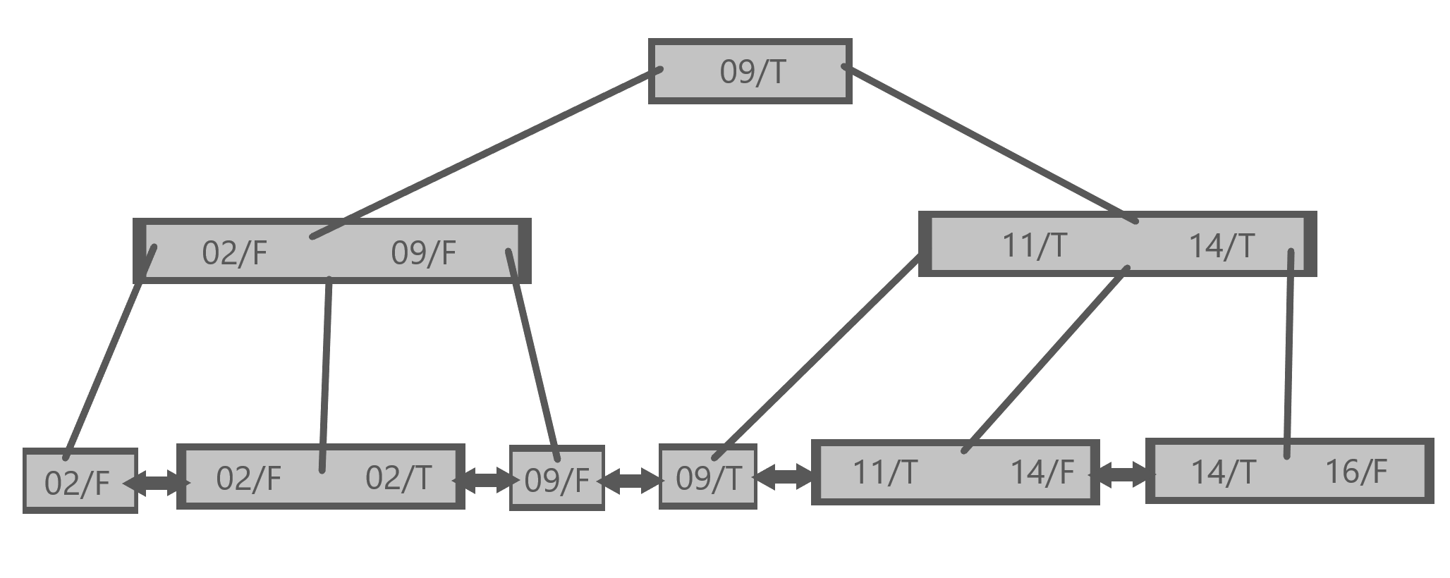
This query filters on two columns, score and official. One thing we could do is to create a compound index on both columns.

B+ Tree representation

Let's do so, placing score first since that's how it is listed in our query. Here is the B+ tree representation:

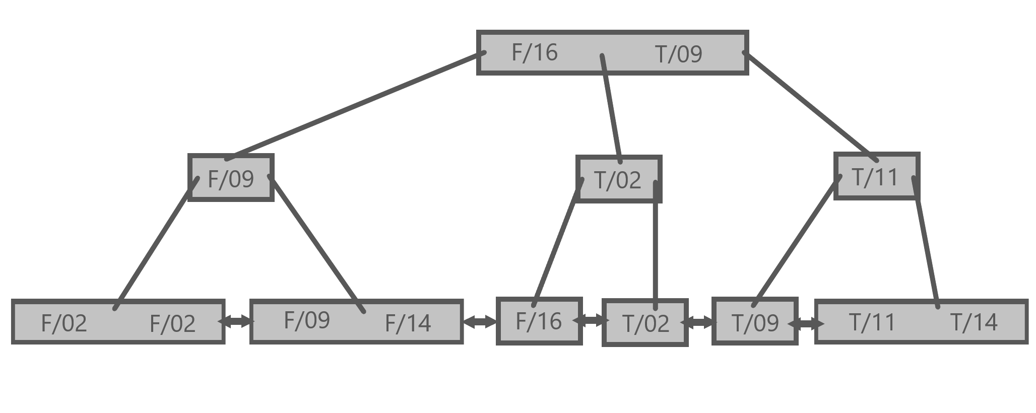
We could instead swap the order and create the index with official first. Here is what that index would look like using the more direct B+ tree representation:

This may make you wonder:

Is one of these indexes better than the other for this query? If so, which one and why?

The answer to that question is:

The second index, which has official first, is absolutely better!

How did we determine that? If we look at the two root nodes, for example, it isn't clear at all if the ( 09/T ) one would be any different than the ( F/16 T/09 ) one.

However when we look more broadly at what parts of the B+ tree are scanned when the query is executed the answer becomes much more apparent!

For the first index, that looks something like this:

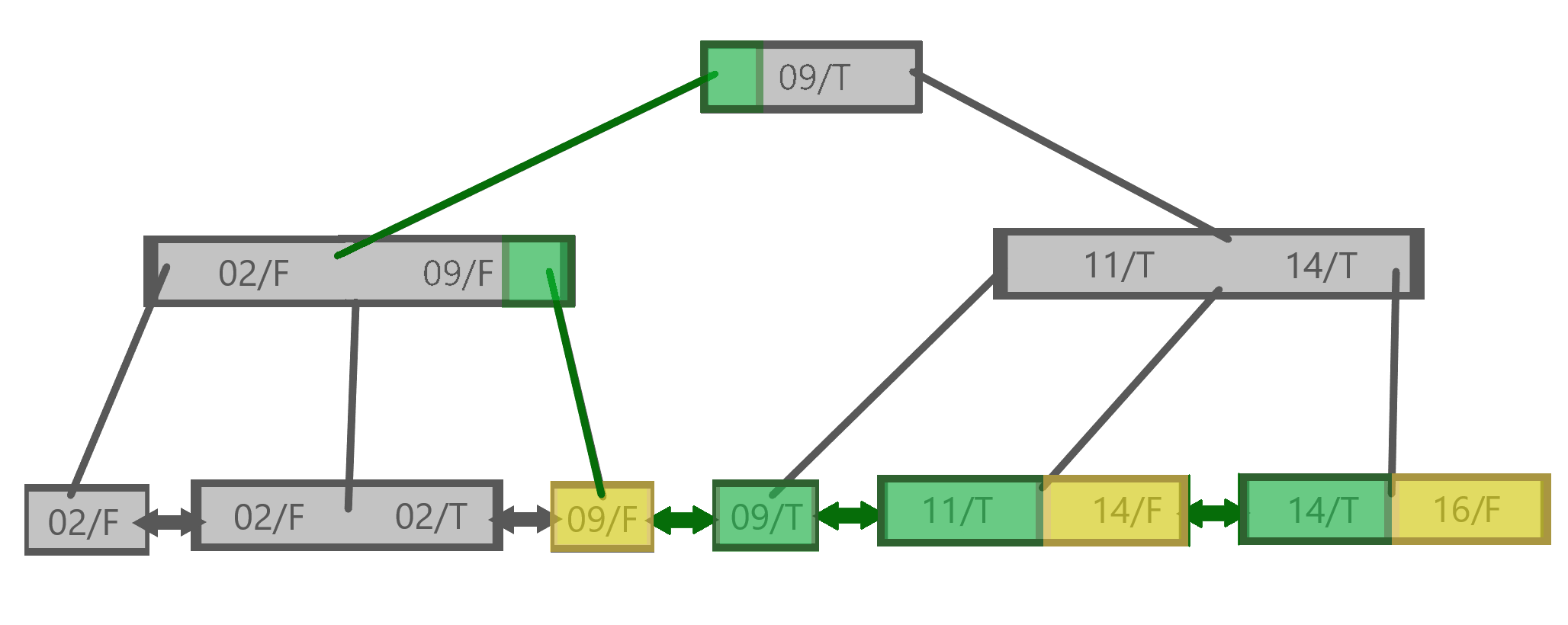
One of the important things to notice here is that the database scanned 6 out of the 9 total leaf nodes. Three of them, shown in yellow, did not match the query.

By contrast, the other index can be used by the database as follows:

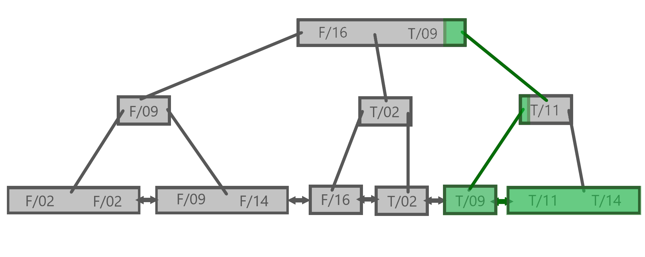
This time around we see that only the 3 leaf nodes that match the query are scanned. The reason it can do this is because the data we are interested in is all located together in one part of the index. We can determine this based on how the index was originally defined, specifically (official, score) in this case, but that is not at all obvious when looking at the B+ tree representation.

IndeX-Ray™ Representation

IndeX-Ray™ represents a better way to 'look' at and reason about these indexes.

Here is the first index of (score, official):

As we mentioned in the intro, the final layer of the index remains the same in this representation. It is only the layers above that which have been shuffled around. In particular these internal layers now separate things out much more:

• A node does not contain multiple entries, such as both 11/T and 14/F as in ( 11/T 14/F )
• Each column in the index, here score and official, has its own layer in the tree. So 11/T would instead be a node with 11 which has a node with T as a child.

Together these changes result in the visualization having subtrees that are more meaningfully defined. We no longer have, for example, a node with O9/T underneath a parent node which has ( 11/T 14/F ). Instead, the internal nodes always share the same values with leaf nodes that descend from them.

When we flip the index definition around to (official, score) we get the following:

We can see a much bigger change between the two IndeX-Ray™ representations than there was between the two B+ tree representations.

It should immediately be clear that the entire subtree of F (false) is not relevant to the query and can be avoided altogether. This is "why" the second index has the data grouped together in a manner that is better for the query. Being able to see this makes it much easier to reason about the layout of indexes and how they can be used.

Takeaways

This article introduced IndeX-Ray™, a technology that allows you to see the indexes inside of databases like never before.

This technology is a powerful tool used by anyone serious about query performance. It allows us to clearly "see" how indexes are used inside of databases. No longer having to guess about the layout of the information unlocks some powerful insights about how to best use them. IndeX-Ray™ turns anyone into a Query Doctor!

Need to go deeper?

• Use IndeX-Ray™ to get a free checkup of your index, no waiting required.
• Check out how indexes can return data directly.
• Subscribe to the newsletter to hear when new articles like this are published and to keep up to date with other exciting announcements.